Monday 13 April 2015

Paralytic Analytics-Statistics of old age

Will you be a sane 80 year old?


I came across this question on quora:

What is the statistical likelihood that a man in his early 70's will comfortably live ten more years, with all mental faculties present?

Let us look at the answer...
You know what? I am just gonna copy paste my answer on the website here...

Assumption: I am assuming that you are an Indian.
The Statistics:

India population -1,282,741,906 (1.28 billion) As of March 28, 2015.
Sex Ratio:
Current Sex Ratio of India 2015 -943 females for every 1,000 males
That means you have a 51.45% chance of being a male.

Age consideration:
India has the following age distribution-
age 65 and above-5.8% (male 34,133,175/female 37,810,599) (2014 est.)
This means that you have a of 2.75% of being a male over the age of 65.

According to @ Facts and figures about mental illness website@ three% of the population faces disability due to mental illness and around 20% of adults are affected by some form of mental disorder every year.

So, lets be a tad bit pessimistic (this sort of also factors in your old age) and say that you have a 20% chance of going senile. The good news is that there is an 80% chance that you wont go senile.

So factoring in all this we calculate:
1,282,741,906 *0.5145*0.0275*0.8=14519355.63
probability=14519355.63/ 1,282,741,906 =0.0113= 1.13%

So there you have it!
There is less than 1.13% chance that you will grow up to be a sane 80 year old.
Please bear in mind that this too is a very generous estimate. A more accurate assessment would depend on other unmentioned factors like religion, social status, income, number of children and their gender, your region of residence, crime rate, lifestyle choices etc. All these factors mostly contribute towards making your chances even slimmer.

Hey! I am not pessimistic; it's just that the answer to your question was almost bound to be a tad bit depressing.
But, look at the brighter side...

The life expectancy of an average Indian is 66.21 years. Which means you are actually really lucky to have crossed the age of 70! So the possibility that you will reach 80 is quite low but if your luck and current age were to be considered as any sort of factors here, then I would say that you are definitely one of the exceptions to the rule.

Remember what they say about life: It's a short trip! Better make it a good one.
Good luck for the rest of your life.

Sunday 5 April 2015

K Means Clustering -Machine Learning

K-Means Clustering in Python (Unsupervised Learning)

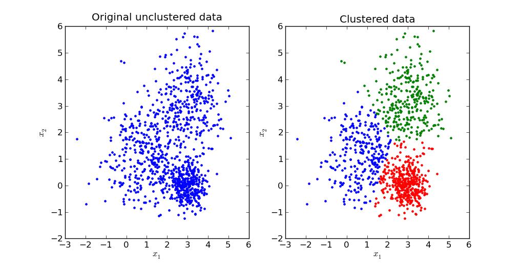
The K-means clustering algorithm is a class of unsupervised learning algorithm that takes an unlabeled dataset and divides it into a user defined number of clusters. These clusters consists of data-points which are more similar to each other than the members of the other cluster.
It can be thought of as a crude form of pattern recognition.
Image taken from the web
 The algorithm can handle any number of features for each data-point but with the condition that all of them are numerical values rather than nominal. Categorical data needs to be converted into binary tags.

Usually playing around with the number of clusters and plotting them for visual verification is a good practice.

The python code has been provided below. You can also download it and all of my other code from my Github page. As always, any improvement or contribution will be appreciated. 
Note: You will need to have pre-installed numpy and pandas libraries before running the code . The program itself is plug and play

The code...

###################################################################


"""K means clustering"""
import pandas as pd
import numpy as np

if __name__=="__main__":
    
    print("welcome to the k means clustering package. this program will help you\n\
    create a user defined number(K) of clusters of similar data points\n\
    the clusters are created based on a crude techineqe of pattern recognition\n\
    This algorithm only works on numerical data\n\
    So lets begin...")
    ####load dataset
    da=raw_input("please mentation the name of your data file (only csv file formats accepted)\n")
    kay=raw_input("how many clusters would you like to create?\n")
    k=int(kay)
    dat=pd.read_csv(da);
    d=np.mat(dat);
    n=d.shape[1]
    m=d.shape[0]
    
    a=1
    b=-1
    cento=np.mat(np.random.rand(k,n))
    cent=a+(b-a)*cento
    
   
    norm=np.mat(np.zeros(shape=(1,n)))
    
    
    #normalization
    for i in range(d.shape[1]):
        norm[0,i]=max(d[:,i])-min(d[:,i])
    nd=np.mat(np.zeros(shape=(m,n)))
    for i in range(n):
        for j in range(m):
            nd[j,i]=(max(d[:,i])-d[j,i])/norm[:,i]
    """for l in range(len(nor)):
        norm[:,l]=nor[l]
    #kMeans(nd,k,cent,distMeas=distEclud)
    m = d.shape[0]"""
    
    clustertag=np.mat(np.zeros((m,1)))
    meansumk=np.mat(np.zeros((1,n)))    
    newcent=np.mat(np.zeros((k,n)))
    box=np.mat(np.zeros((k,n)))
    #print norm,nd
    while 1:


        for i in range(m):
            
            box[:,:]=d[i,:]
            #print box
            sqdif =np.power((box-cent),2)
            root=np.power(sqdif,0.5)
            rsum=root.sum(axis=1)
            indexleast=np.argsort(rsum,axis=0) 
            clustertag[i,0]=indexleast[0]
            print indexleast


        for i in range(k):
            count=0
            for j in range(m):
                if clustertag[j,0]==i:
                    meansumk[0,:]=meansumk[0,:]+d[j,:]
                    
                    count+=1
                    newcent[i,:]=meansumk/count
        cent=newcent
        if newcent.all()-cent.all()==0:
            break
    
    lom=np.mat(np.zeros((k,n)))
    print ("The centroids of the %i clusters are...\n"%k)
    for h in range(k):
        lom[h,:]=np.multiply(norm[0,:],cent[h,:])
    print lom

##############################################

What the input should look like
What the output would be like...

The output will be a matrix of K number of rows representing the centroid of the each cluster. You can also think of it as an average feature vector of that particular cluster.

K Nearest Neighbor Algorithm -Machine Learning

Classical K-Nearest Neighbor Algorithm in Python

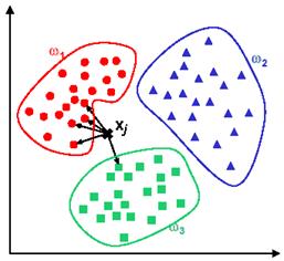
The K-nearest neighbor algorithm is a supervised learning algorithm used to classify data-points based on multiple features. It can handle both qualitative and quantitative data. The core logic of the algorithm is to compare the new data point to all the existing data-points in it's database and assign it to the group which it most resembles. Apart from the dataset, the algorithm also requires the user to define a parameter 'K'. To understand why this parameter is needed, one must have at-least a rough idea of the inner workings of the algorithm.
Image taken from the web


What the algorithm basically does is it sorts every data-point in it's database according to decreasing degree of similarity to the new data-point. Now, this sorted list may have points from every class of the data-set; so, to give a "best guess" answer of the classification problem, it takes a vote. For this vote it chooses the top K items in the list and assigns the new data-point to the class which has a majority in this population. A good value of K usually depends on the size of the population and for large data-sets, it is enough to choose a K at around 10% of the total population.


It's application may range anywhere from segregating customers of a supermarket into different categories to writing software for solving captcha autonomously.
Example of a captcha (taken from the web)
The python code for this algorithm has been given below (I use the Spyder IDE).You can also download it from my Github page. Any contribution and  improvement to the code is duly welcome. The code is plug and play.

Note: Apart from the standard python packages, you will also need numpy and pandas to use this code.


The code...
############################################################################
import numpy as np
import operator
import pandas as pd


if __name__ == "__main__":
print ("Welcome to K-nearest neighbor supervised learning classifier.\n\
All you will need to do is give your dataset and your unclassified feature set and this program will classify it for you\n\
Please keep in mind that the data must be in a csv file or else you will have to modify the source code\n\
\n\
so lets begin...")

da=[]
mother_file=raw_input("please mention the name of your mother file\n")
da = pd.read_csv(mother_file)
d=np.mat(da)
dataset=d[:,0:-1]
labels=d[:,-1]


inx=raw_input("please enter your input parameters in the form of a list ")

x=np.mat(inx)
if x.shape[1]!=dataset.shape[1]:
print ("invalid input\n please run the program again")

kay=raw_input("how many nearest neighbours(k) would you like to count the majority from\n")
k=int(kay)
siz=dataset.shape[0]
bl=np.zeros([dataset.shape[0],dataset.shape[1]])
for i in range(len(bl)):
bl[i,:]=x
difmat=bl-dataset

sqdifmat=np.square(difmat.astype(float))
root=np.sqrt(sqdifmat)
distances = root.sum(axis=1)

sortedDistIndicies = np.argsort(distances,axis=0)
classCount={}

for i in range(k):

voteIlabel = labels[sortedDistIndicies[i]]
classCount[voteIlabel] = classCount.get(voteIlabel,0) + 1
sortedClassCount = sorted(classCount.iteritems(), key=operator.itemgetter(1), reverse=True)
print sortedClassCount[0][0]

##############################################################

How to format the data...
For the code to work without you needing to poke around the script itself, your data needs to be stored in a .csv file. The given code can handle alphanumeric designation of the class but its feature description needs to be strictly numeric.
Something like so...
The code can handle an arbitrary number of features and does a better job than the Matlab code seen before on this blog.
Remember, the input that you give to the algorithm must be in the form of a list.

Saturday 28 March 2015

Machine Learning-Artificial Neural Networks

Artificial Neural Network - With Back-propagation Algorithm(Supervised Learning)

Artificial neural networks  are basically a bunch of computer code that tries to learn from given examples.
A skilled practitioner of machine learning can use artificial neural networks (ANN's) to teach a computer to do virtually anything. Many respectable researchers in the field believe to be the panacea algorithm; the one algorithm for solving every hard problem (in a certain- narrow sense of-course !)
image taken from the web


Neural networks have been around for quite some time now but they  still are a topic on which massive amounts of research is ongoing.

The whole idea behind a neural net is to mimic the brain. The argument is that,  like an average Joe who can master multiple languages and skills during his lifetime using the same set of neurons in his brains (it's not as straightforward as that- but what the hell) the same algorithm which tries to mimic the biological neurons should be able to learn anything if used properly.

ANN based applications are ubiquitous now-a-days and it is an important tool to to add to your repertoire as an analyst.

Writing code for an ANN is relatively straightforward; using it effectively on the other hand is somewhat of an art. It takes time , patience and practice.

I have provided below the python code (Yes python, I guess it was time to switch from MATLAB)  for an artificial neural network which trains using the back-propagation algorithm.  The code is plug and play but as a user, you are expected to know how to use a neural network. The finer points have been mentioned below. You can also download the code from my Github page. As always, contributions to the code are welcome and appreciated.


Additional Requirements- Numpy (I use the Spyder IDE)


The code:
##########################################################################3

import numpy as np

def sgm(x,derivative=False):
if not derivative:
return 1/(1+np.exp(-x))
else:
out = sgm(x)
return out*(1.0-out)

def linear(x,derivative=False):
if not derivative:
return x
else:
return 1.0

def guassian(x,derivative=False):
if not derivative:
return np.exp(-x**2)
else:
return -2*x*np.exp(-x**2)

def tanh(x,derivative=False):
if not derivative:
return np.tanh(x)
else:
return (1.0-np.tanh(x)**2)


class backPropagationNetwork:
layerCount = 0
shape = None
weights = []
layerTransferFunc = []

# constructor function for the class
def __init__(self, layerSize,layerTransferFunc = None):
# layerSize is the Architecture of the NN as (4,3,1)
self.layerCount = len(layerSize)-1 # input layers is just a buffer
self.shape = layerSize

# for the forward pass maybe.
self._layerInput = []
self._layerOutput = []
self._previousWeightDelta = []


for(l1,l2) in zip(layerSize[:-1],layerSize[1:]):
self.weights.append(np.random.normal(scale=0.1,size=(l2,l1+1)))
# add for each weight matrix a matrix in _previousWeightDelta for previous values
self._previousWeightDelta.append(np.zeros(shape=(l2,l1+1)))

if layerTransferFunc is None:
layerTransferFunc = []
for i in range(self.layerCount):
if i == self.layerCount - 1:
layerTransferFunc.append(linear)
else:
layerTransferFunc.append(sgm)
else:
if len(layerTransferFunc) != len(layerSize):
raise ValueError("Incompatible no of transfer functions.")
elif layerTransferFunc[0] is not None:
raise ValueError("no transfer functions for input layer.")
else:
layerTransferFunc = layerTransferFunc[1:]

self.layerTransferFunc = layerTransferFunc


# forward run/pass
def run(self,X):

# no of training examples
m = X.shape[0]

# initialize/ clear out the input and output list from previous run
self._layerInput = []
self._layerOutput = []

# Forward pass
for i in range(self.layerCount):
if i == 0:
layerInput = self.weights[0].dot(np.vstack([X.T, np.ones([1,m])]))            # vstack(a,b) stacks matrix/vector b below matrix/vector a
else:
layerInput = self.weights[i].dot(np.vstack([self._layerOutput[-1], np.ones([1,m])]))

self._layerInput.append(layerInput)
self._layerOutput.append(self.layerTransferFunc[i](layerInput))

return self._layerOutput[-1].T


def trainEpoch(self,X,Y,trainingRate ,momentum ):
# trains the network for one epoch
delta = []
m = X.shape[0]

# forward pass before we can compute the gradient by back propagation
self.run(X)


for i in reversed(range(self.layerCount)):                                             # reverse as the backpropogation work in reverse order

if i == self.layerCount-1:                                                         # if this is for the preactivation at the output
outputDelta = self._layerOutput[i] - Y.T                                      # this is also the gradient at output if we take the least square error function
error = np.sum(outputDelta**2)                                                # sum of all the elements along all dimensions
delta.append(outputDelta*self.layerTransferFunc[i](self._layerInput[i],True))                  # '*' operator is for coordinate wise multiplication
else:
deltaPullback = self.weights[i+1].T.dot(delta[-1])  # this is the gradient at the activation of the hidden layer (i+1), note that i = 0
 # is for hidden layer 1.
delta.append(deltaPullback[:-1,:]*self.layerTransferFunc[i](self._layerInput[i],True))         # this is the gradient at the preactivation at hidden layer (i+1)

for i in range(self.layerCount):
deltaIndex = self.layerCount - 1 - i # delta[0] is preactivation at output and so on in backward direction
if i == 0:
layerOutput = np.vstack([X.T,np.ones([1,m])]) # for W0 the delta (preactivation) is input layers
else:
layerOutput = np.vstack([self._layerOutput[i-1],np.ones([1,self._layerOutput[i-1].shape[1]])]) # _layerOutput[0] contains the activation of the hidden layer 1 and so for Wi we need _layerOutput[i-1]

weightDelta = np.sum(layerOutput[None,:,:].transpose(2,0,1)*delta[deltaIndex][None,:,:].transpose(2,1,0),axis=0)

weightDelta = trainingRate * weightDelta + momentum*self._previousWeightDelta[i]
self.weights[i] -= weightDelta
self._previousWeightDelta[i] = weightDelta

return error # incase useful


if __name__ == "__main__":
 
    print ("welcome to neural network")
    data_file=raw_input("please mention the name of your training set file\n")
 
    d=np.genfromtxt(str(data_file),delimiter=',')
    z=np.shape(d)
    print ("your data set has %i datapoints a\n"%z[0])
    print ("And there are %i columns\n"%z[1])
    nx=int(raw_input("how many of the %i columns are inputs ?\n"%z[1]))
    ny=z[1]-nx
    x=[]
    y=[]
    for p in range(z[0]):
        x.append(d[p,0:nx])
        y.append(d[p,nx:])
    X = np.array(x)
    Y= np.array(y)
    net_def=[int(nx)]
    print net_def
    qwe=raw_input("how many epochs ?\n")
    hlc=int(raw_input("how many hidden layer do you want ?\n"))
    print int(hlc)
    for n in range(int(hlc)):
        a=raw_input("how many units in layer %s\n"%(n+2))
        net_def.append(int(a))
    net_def.append(ny)
    m=float(raw_input("please define momentum:\n"))
    alph=float(raw_input("please define learning rate:\n"))
    print("You can choose from a host of transfer functions :-sigmoid(sgm),linear(linear),gaussian(gaussian),tanh(tanh)\n")
    tff=str(raw_input("choose on of the transfer functions(mentioned in paranthesis above)\n"))
    tup=tuple(net_def)
    layerTransferFunc = [None]
    for n in range(len(tup)-1):
        layerTransferFunc.append(str(tff))
    bpn = backPropagationNetwork(tup)
    maxIteration = int(qwe)
    minError = 1e-5
 
    for i in range(maxIteration+1):
     
     
        err = bpn.trainEpoch(X,Y,momentum=float(m),trainingRate=float(alph))
     
        if i%100 == 0:
            print "iteration {0}\t error: {1:0.6f}".format(i, err)
        if err <= minError:
            print "Minimum error reached as iteration {0}".format(i)
            break
    Ycomputed = bpn.run(X)
    for i in range(np.shape(X)[0]):
        print "Input: {0}\n Output: {1}".format(X[i],Ycomputed[i])#tup
    print(bpn.shape)
    print(bpn.weights)


########################################################################


How to use : This is the art part.

First of all, your data should be munged properly on a spreadsheet with normalized decimal values and binary tags and subsequently be saved as a .csv file or a text file.

Next, as always, all your initial columns must represent the inputs to the neural network and the rest have to represent the corresponding output (remember that we are doing supervised learning). Every row is one data point i.e. one training example. The program will ask you for these when you run it and based on that, it will decide the number of nodes in the input and output layer.

It will then ask you about the number of hidden layers and the number of nodes in each layer.
You will also be prompted to define the learning rate and momentum; both of which are values between 0 and 1.

You will also be asked to decide the number of epochs . Epochs is just a fancy way of depicting the number of times the algorithm uses your entire dataset to train the network. It is usually in the order of millions.

The learning rate is somewhat analogous to the size of steps that you want to take while trying to solve an optimization problem and the momentum can be intuited as a coefficient that decides the amount of impact that the already learnt parameters will have on the subsequent learning steps. You may also need to decide if you have sufficient data. In machine learning , more data is almost never a bad thing (if you are willing to compromise on the computational cost front).

Deciding the network architecture (number of hidden layers and their nodes) and cleverly choosing inputs and outputs along with fine-tuning your learning rate and momentum parameters may take some time and experimentation. It is all about finding the right balance . After the error converges to a level of you satisfaction, you can use the network for doing further prediction/classification/regression etc.

All you have to do is declare your new input vector as a numpy array (lets call it "R") and write the folloing in the command window :-
#################
Y=bpn.run(R)
print Y
###################

you can also print the weight matrix by using the following command:-
##########
print weights
###########

Acknowledgements:
I must thank the following two people who unknowingly helped me create this post:
This Amazing Person's Youtube tutorial and
This like minded fellow programmer's Github page
                                         

Monday 23 March 2015

Paralytic Analytics-Epidemics

How To Create An Epidemic -Using Logic and Psychology 


                                                     THE DEVIL IS IN THE DETAILS

Most people think that the job is of an analyst is  just to passively analyse the information that he gets and produce useful insights using that. Well that is only half the truth. Sometimes you may be asked to proactively exploit your understanding of a system to create the desired effect. 

In his book The Tipping Point: How Little Things Can Make a Big Difference by Malcom Gladwell the author has describe how epidemics, in every sense of the word are created. Epidemics ranging right from the flu to a fashion or opinion epidemic. He, in very vivid detail describes what it takes to make something go viral; and not just in the context of the internet.

Here is a resipy of a strategy for creating a useful epidemic.
Lets look at it from the eyes of a Mathematician and Game theorist.

The best way to learn is by example. Suppose you the owner of a alternate energy solutions company which specializes in solar micro-grid based solutions. Now like any other business, your main aim is to make the maximum possible profits. And there are four main ways of making a lot of money while selling something.
Either...


  • you should have a monopoly over the sale of the goods/services that you are selling or
  • your product should be the best in the market in which case it can be difficult to offer a competitive price , or 
  • you have to sell something extremely precious and it's price should not be regulated by any organisation, that means that you cant sell oil or gold but one of the many viable options is art. But sadly you ended up in the energy business so that is off the table. And finally
  • you should sell something in huge volumes with a small margin for profit. That way you increase your probability of being liked by a larger crowd of people and the probability of repeat customers because of the competitive pricing that you are able to offer.

Well , you may have the best product in the market , in which case you don't need to read further but we are looking for a way of creating a successful business independent of the kind of product that you are offering. Of course , product quality does matter in the long run, but that is not the only factor.

That narrows down your options to just one- maximizing your sale volume.
So how to maximize sale volume you ask?
Well, the answer to that is simple (but not trivial); first o fall you need find a target customer base.

Your target customer/client base is a group should have the following properties:


  • They should be one of the majority sections of the society.(Because you want a lot of clients)
  • Should be able to afford your services/product and will benefit from it.

That narrows it down to everybody starting from the middle class and above who lives in a house and even other companies that have office buildings of any sort. Now one other thing that you need to be aware of is the limitations of your product. you cant go around making false promises. And you need to tell your clients about it in the most strategic way. Something on the lines of "No, no Sir, your wife is not fat at all, she is just Not Thin".

One obvious client base in your target city for business lives in the suburbs and housing colonies. So basically you are looking for similar people (socially and economically) who live in close proximity.

Now, the "game" begins...

The book Tipping point describes three main factors that are important for triggering an epidemic

1. "The Law of The Few". Unlike what most of you may be thinking, epidemics depend on a select group of very few people. They are of the following 3 types :-


  • The Connectors: These are the people in a community who know large numbers of people and who are in the habit of making introductions. A connector is essentially the social equivalent of a computer network hub. They usually know people across an array of social, cultural, professional, and economic circles, and make a habit of introducing people who work or live in different circles. They are people who "link us up with the world...people with a special gift for bringing the world together". They are "a handful of people with a truly extraordinary knack for making friends and acquaintances".Malcolm Gladwell characterizes these individuals as having social networks of over one hundred people. Gladwell attributes the social success of Connectors to the fact that "their ability to span many different worlds is a function of something intrinsic to their personality, some combination of curiosity, self-confidence, sociability, and energy".
  • The Mavens: These are "information specialists", or "people we rely upon to connect us with new information". They accumulate knowledge, especially about the marketplace, and know how to share it with others. Gladwell says "A Maven is someone who wants to solve other people's problems, generally by solving his own". According to Gladwell, Mavens start "word-of-mouth epidemics" due to their knowledge, social skills, and ability to communicate. As Malcolm Gladwell states, "Mavens are really information brokers, sharing and trading what they know".
  • The salesmen: These are "persuaders", charismatic people with powerful negotiation skills. They tend to have an indefinable trait that goes beyond what they say, which makes others want to agree with them.

2. The stickiness factor. The specific content of a message that renders its impact memorable. This may include the use of catch phrases or slogans. Something on the lines of the Tata Sky catch phrase , "Isko laga dala to life jhingalala"


3. The power of context. Human behavior is sensitive to and strongly influenced by its environment. As Malcolm Gladwell says, "Epidemics are sensitive to the conditions and circumstances of the times and places in which they occur". This will be better understood as you read further.

Malcom Gladwell is not the only one teaching about how you can make things more popular instantly. An interesting way of looking at this methodology can also be seen in one of the lectures on "Learning:Near misses, Felicity Conditions" by MIT's Patrick H Winston in his artificial intelligence lecture series. He proposes the method of inducing felicity to any product using the five factors represented on a star.(The 5 S's)


Here is a breakdown of the five features that your product/idea (basically anything that you are trying to sell) should have:


  • Symbol: This is as simple as it looks. Your product/idea should be represented by a visual handle like a brand icon that reminds people of your product/idea every time they see it. This accounts for a vast majority of the crowd who are visual thinkers.
  • Slogan: This is again a sensory handle for the people to be reminded of your product/idea . The slogan you create should have the stickiness factor in it, ergo, once people hear it, they should not be able to take it off their mind. This is where Gladwell and professor Winston meet.
  • Salient Thought: Well this is a bit tricky to understand and implement, but when you think about the salient feature of your product/idea , it usually refers to the feature that really sticks out without it being directly mentioned. It basically pertains to the purpose of the particular endeavor. For example; what is the salient thought of a Fort ? It is security during a siege. This needs to be clearly conveyed by your selling pitch.
  • Surprise: This pertains to the uniqueness of your idea/product. The surprise factor usually demands a deviation from the norm in such a way that it has never been seen or expected before. All this may take a certain level of showmanship on your part. And finally
  • Story: See, people just LOVE a story. Studies have shown a heightened retention of stated facts in an average person if they are presented to them in form of a story. Stories are sort of a mnemonic device for remembering facts.

So, there you have it, if you can execute the above five steps perfectly, it is virtually guaranteed that your product/idea will be widely appreciated.

And now you may ask that all this may be good in theory, but how do you really go about doing all this.
To understand that, we come back to our solar energy solutions example.

Most of the features suggested by Prof. Winston may be handled by marketing and or consulting firms, but we will now see what can be done on a human level for ensuring success in your business.

The first thing you need to arrange for are the salesmen . They are the ones that will be doing most of the legwork for you.
Once you have your guy and I am trusting your judgement of character for choosing one, you move onto the next step.
You have to find the connectors and the mavens and that to simultaneously. This is when you put your salesmen to work.

Here is how you identify your connectors:
They are the famous people who live in your targeted suburb. They may be the heads of the community, local political leaders and pseudo-celebrities. But keep in mind that they cannot be too different from your target audience, they just have to be respected members of the society whose abode is frequented by very many. These people will form the focal point of your expansion campaign.

It is these people that you need to sell your product to first and do so in such a way that it is amply conspicuous . For example, although it is normal practice to just place solar panels on the roof of the building and be done with it but in this case you may need to make an exception. The installation (even if temporary) need to be visible for miles around. Maybe you can install the solar panels on elevated platforms on the roof for no added cost for the period of you epidemic campaign and later "upgrade" to the more safer mode of just placing the panels on the roof floor. The purpose of this " peacock display " is to force the visitors to the connector's place to talk and ask about their recent acquisition. This will help to trigger the first kind of epidemic that you need to generate - The word of mouth epidemic.

Now you need to find your mavens:
It is preferable that your connectors double as mavens, i.e. they display a keen knowledge about the benefits of the recent addition to their home/office. But you don't need to worry about that because people like the feeling that they have made a good decision after it becomes irreversible. So you can rely on your connectors for becoming maven who have expert advice to share which was provided by your salesmen in the first place.

The second principle of psychology that you can exploit for your epidemic campaign id the principle of social proof and authority. So apart from the newly wise connectors , you need to find people who hold a certain sway over their neighbors and society by virtue of their technical knowledge about your product. These may be engineers , owners of technical businesses or related to anything even tangentially related to technology and not necessarily your technology. These people are prone to give free advice as a tribute to their astute technical knowledge. you need to first convince these people about the greatness of your product, because these are the people to whom their neighbor goes for advise after the visit to the connector's place to validate his prospective investment in your product.

It is like so :- if a doctor (assume he is a pervert) asks you to strip in-front of him for the medical checkup though you know that it is only a bruise on your hand and does not warrant a full body inspection, you will still consider the idea of consenting to strip because after all , he is a doctor, and knows better, so you better strip or die because of the mysterious prognosis he may not find if you don't strip. So you depend on his authority and trust him to have only the best of intentions. So, you believe anything he says.

This is what you are trying to achieve through converting the techies in the target crowd into clients.
The other psychological weapon that you are using is of social proof. "If all the important people are buying this product , then it must be awesome. So I am going to buy it too".

The other socio-psychological effect that is desirable is that of forced stickiness and it also borrows concepts form the concept of power of concept. This you can achieve by conducting an aggressive yet cheap ad campaign wherein people see you ads everywhere they go. This may include inserting flyers in the daily newspaper that everybody subscribes to and sticking them in places like building elevators and anywhere else that you can imagine. This will help boost your stickiness factor by exposing people to your brand symbol and slogan again and again.

This is how you influence a large section of society using a very few people. After this it is just about following the savage civilization approach. You move from suburb to suburb and from city to city , sucking up clients and leaving behind a trail of profit in your wake.


So there you have it, a full blown cook book approach to creating your own epidemics !

Understand, that these strategies are universally applicable with slight adjustments with respect to context.


Thursday 5 March 2015

Anomaly Detection - Machine Learning

Anomaly Detection Algorithm (Supervised Learning)

Anomaly detection is an algorithm that uses a huge dataset of healthy examples to learn about the features of the average good example and then uses the metrics learnt to compare with a new example and decide as to whether the new example is an anomaly to the commonly witnessed specimens.

As an analyst , one example where you may use this algorithm is to detect anomalous visitors to your website by looking at factors like number of visits per day, number of posts in the forum and typing speed. 
Another example may be in a server room/ data center where you may predict system failure by detecting anomalous activity in features like CPU load, number of disc accesses per second, memory usage and CPU load per unit network traffic.


The above two figures show a surface plot of a Gaussian variable dependent on two parameters x1 and x2.

Data Representation

The dataset should be in the form of a .csv file or a similarly syntaxed text file.

The algorithm assumes that your data-points have a normal (Gaussian) distribution.
The Matlab code has been provided below. It is pretty much just plug and play. You can also download the code from my Github page. Any suggestions and contributions will be duly appreciated.

A few things to keep in mind...
  • The code can handle any number of features but as always , they have to be numerically describable.
  • The algorithm asks you to choose a normalized threshold parameter i.e. a value between 0 and one. The general rule of thumb is that the more particular you are about the spread of your data, the higher should be your threshold. In other words, if a very narrow margin of error is allowed in your healthy examples, then you should choose a very high value of threshold. It is sort of like a quality scale where 0 being the worst quality and 1 signifying the best quality.
The code...
####################################
% anomaly detection
fprintf('welcome to the anomaly detection module\n');
fprintf('the dataset that you will use to train the algorithm');
fprintf(' must only have non anomalous examples \n');
da=input('please mention the dataset file in single quotes: \n');
x=load(da);
s=size(x);
l=s(1,1);
b=s(1,2);
fprintf('your dataset has %i healthy examples with %i features \n',l,b);
fprintf('training...\n');
mus=zeros(2,b);

for i=1:l
    for j=1:b
        mus(1,j)=sum(x(j,:))/l;
        mus(2,j)=(1/l)*var(sum(x(j,:))/l,x(j,:));
    end


end
fprintf('training complete.\n');
inp=input('please enter new datapoint for checking if it is anomalous :\n');
eps=input('please enter normalized threashold probability :\n');
p=prob(inp,mus);

if p<eps
    fprintf('this dat-point is an anomaly\n');
end

if p>eps
    fprintf('this data-point is healthy\n');
end


###############################

Save the following function as 'var.m' in your working directory.

#####################
function x=var(a,b)
for i=1:length(b)
    c=(b(1,i)-a)^2;
end


x=(1/length(b))*c;

end
###############

Save the following function as 'prob.m' in your working directory.

####################
function p=prob(a,b)
p=1;
c=zeros(1,length(a));
for i=1:length(b)
    c(1,i)= (0.3989*(1/sqrt(b(2,i))))*exp(-((a(1,i)-b(1,i))^2)/2*b(2,i));
end
for j=1:length(a)
    p=p*c(1,j);
end
end
##################


Tuesday 3 March 2015

K-Nearest neighbors Algorithm - Machine Learning

K-Nearest Neighbors Algorithm-Vector style ( supervised learning)


The K-nearest neighbor algorithm is a supervised learning algorithm where the computer learns how to classify new data-points based on the training examples that you give it.

This algorithm can handle any number of categories unlike the logistic regression classifier .

Let us see what it does using an example...
Suppose you have to classify data into multiple categories based on any number of features. For illustrative purposes, we shall look at just two features.
The figure shows clusters of four categories (red ,green ,blue and brown) and their centroids plotted against two arbitrary features.

Now we need to find out which category the new point belongs to. This can simply be done by comparing the vector component of the new point on the centroid vectors of the four clusters. The cluster centroid on which the new point's vector subtends the largest component can safely be assumed to be the parent category.

For this algorithm, I am giving the Matlab code below. You can also download from my Github page.

Data format

  • Your training data can be in the form of a .csv or a similarly syntaxed text file.
  • Your complete dataset should consist of features which are NUMERICALLY DESCRIBABLE and only the last column of your dataset must contain the decimal category label.
  • You should know the total number of categories that your dataset depicts.
The code...


###############################################
% k nearest neighbours vector style

fprintf(' welcome to the vector style k nearest neighbour module\n');
da=input('please mention the dataset file in single quotes :\n');
d=load(da);
s=size(d);
l=s(1,1);
b=s(1,2);
fprintf('there are %i datapoints with %i dimensions\n',l,b-1);

K=input('how many categories are depicted by your dataset?');
x=d;

group=zeros(1,b-1);
centroids=zeros(b-1,K);
 temp_avg=zeros(b-1,K);
 count=0;
%determining the centroid vector for each class
for j=1:K
for i=1:l
    if x(i,b)==j
         
        temp_avg(:,j)=temp_avg(:,j)+x(i,1:b-1)';
        count=count+1;
        group(1,:)=(1/count).*temp_avg(:,j);
        centroids(:,j)=group;


    end
end
end

fprintf('the following are the centroids of the %i categories\n',K);
disp(centroids);
test=input('you can now classify new vectors.\n please enter the new vector :');
component=zeros(1,K);
for i=1:K
    component(1,i)=magnitude(test)*cosine(test,centroids(:,i));
end

 [max_value, index] = max(component(:));
 y=index;
 fprintf('the vector that you want to test belongs to category : %i\n;',y); 


##################################################

save the following function as 'magnitude.m' in the working directory.

############################################
function x = magnitude(a)
x=sqrt(sum(a.^2));
end

##########################################

save the following function as 'cosine.m' in the working directory

####################
function x=cosine(a,b)

c=sqrt(sum(a.^2));
d=sqrt(sum(b.^2));
x=dot(a,b)/(c*d);

end

###################